A Second-Order Side-Channel Attack on Masked Kyber768

Part 3 of the Ledger Donjon series on side-channel attacks against post-quantum cryptography.

In Part 1, we recovered an ML-KEM secret key from an unprotected pqm4 implementation with a textbook Correlation Power Analysis (CPA). In Part 2, we broke the unprotected CRYSTALS reference implementation with a non-profiled deep-learning attack.

This third chapter asks the natural next question: what happens when the implementation fights back?

The target this time is masked Kyber768, or ML-KEM-768. Masking is the standard algorithmic countermeasure against side-channel attacks, and at first order it works exactly as intended: looking at any single sample, the secret disappears into noise. But the leakage does not vanish. It is split between the shares. With the right combiner and the right model, a second-order CPA brings the secret coefficient back.

Before you dive in

• We target mkm4, a first-order masked Kyber implementation for ARM Cortex-M4 described in ePrint 2022/058.
• Masking erases first-order leakage: each secret coefficient is split into random shares, and each share is uniformly independent from the secret.
• Each share still leaks on its own. That per-share leakage is not enough to recover the key, but it gives the attacker two physical signals to combine.
• The centered cross-product exposes second-order leakage. A naive Hamming-weight model does not; the attack needs a mask-averaged covariance model.
• In our experiment, the correct coefficient reaches rank 0 after about 200 traces once the joint point of interest and the leakage model are known.

What is masking?

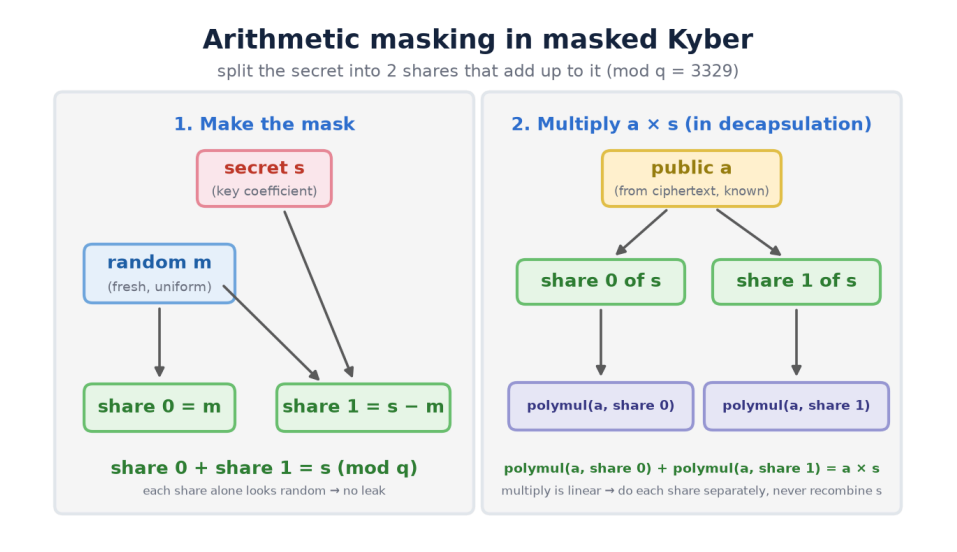
Masking is built around a simple rule: do not manipulate the full secret directly.

Instead of processing a secret coefficient s, the implementation splits it into random arithmetic shares modulo Kyber’s prime q = 3329:

s = s0 + s1 (mod q)

The first share s0, also called the mask m, is drawn uniformly at random for each execution. The second share is computed as:

s1 = s - s0 (mod q)

Each share alone is uniformly random. It carries no information about s. Only the pair (s0, s1) reconstructs the secret, and the implementation is designed so that this reconstruction never appears as a processed value.

Masking in mkm4

We used the same side-channel setup as in the previous posts: the same electromagnetic probe and the same STM32F4 target class. The difference is the implementation. Instead of the unprotected pqm4 code, we attack mkm4, the masked Cortex-M4 Kyber library.

The secret key is carried in Number Theoretic Transform (NTT) form as two arithmetic shares throughout decapsulation. For the base polynomial multiplication, the public input is common to both computations, while the secret remains split:

public * s = public * s0 + public * s1

The device computes public * s0 in one operation and public * s1 in a separate operation, each under its own trigger. The unmasked product public * s is never formed.

We therefore capture two trace segments for each execution: the share-0 window and the share-1 window. For the leakage-detection phase, we captured 100,000 executions.

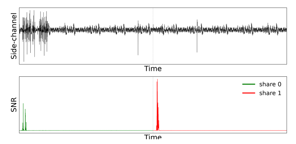
Does the mask hold? First-order analysis

First, we check whether masking does what it promises against a first-order attacker, meaning an attacker who looks at each time sample independently. In this scenario, we fix the mask generation to a known value and generate random secret and public values on each iteration.

Our detection tool is the Signal-to-Noise Ratio (SNR). We group traces by a sensitive intermediate and ask whether the average electromagnetic signal at a sample depends on the group. A high SNR means the sample leaks; an SNR near zero means it does not.

For the first-order check, we use the unmasked secret product as the class label:

HW(montgomery_reduce(public * s))

We compute this SNR across every sample of both share windows.

The result is exactly what masking should deliver: flat noise. No individual sample’s mean depends on the secret. The first-order CPA from Part 1 is dead on arrival.

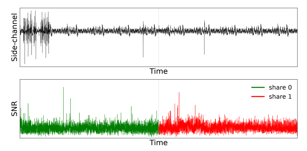
The leak is still there: first-order SNR per share

Masked does not mean silent. The shares are real values, physically computed and moved by the chip. Each share can still leak its own value, even though a single share tells us nothing about the key.

To see this, we change the SNR class label. Instead of the unmasked product, we label each share window by the value processed in that window:

HW(montgomery_reduce(public * s0))
HW(montgomery_reduce(public * s1))

The first label is used over the share-0 window, and the second over the share-1 window.

Now the peaks are obvious. Each share leaks clearly at well-defined samples. Masking has not removed the leakage; it has divided it.

The masking guarantee still holds, because neither share independently reveals the secret. To recover the key, we need to combine information from both windows.

Combining the shares: second-order analysis

A second-order attack looks at two points in time at once: one sample from the share-0 window and one sample from the share-1 window. It then combines them into a single value per trace.

This is the attacker’s tradeoff against masking: the leakage is weaker and the search space is larger, but the dependence on the secret can reappear in the joint behavior of the shares.

Two classic combiners are used in practice:

• Centered cross-product: (x - mu_x) * (y - mu_y), where mu_x and mu_y are the per-sample means. This measures how the two leakages co-vary.
• Absolute difference: abs(x - y). This is a simpler heuristic, historically common against hardware and Boolean masking.

For this attack, the centered cross-product is the useful combiner.

The secret reappears

We compute the centered cross-product across the two share windows, then compute its SNR against the correct model of the secret. This produces a clear second-order leakage peak.

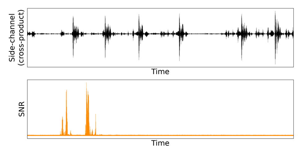
The joint point of interest combines one sample from each share window. Neither sample leaks the secret alone, but their centered product does.

Why the simple Hamming-weight model fails

This is the subtle part of the attack.

For the unprotected target and for the per-share SNR, the leakage model is straightforward:

HW(montgomery_reduce(public * s))

It is tempting to reuse that model for the second-order cross-product. We tried it. It fails: the SNR at the true point of interest collapses to the noise floor.

The reason is structural. The measured value is now a centered product, so its expected value is a covariance between the two share leakages. That covariance is not determined by the Hamming weight of the unmasked product.

Two traces with the same HW(montgomery_reduce(public * s)) can have different expected cross-products. Conversely, two traces with different Hamming weights can have the same expected cross-product. If we bin by Hamming weight, we hide the signal inside the groups instead of separating it between them.

This is the core lesson from the statistical analysis of second-order DPA by Prouff, Rivain and Bevan.¹ The best prediction for a centered second-order leakage is the conditional expectation of the combining function, not necessarily the Hamming weight of the sensitive value.

There is also a practical trap: when the public input is zero, public * s = 0 for every secret. All those traces fall into the HW = 0 group. Since the public value itself is processed in the trace, this can create a spurious peak unrelated to the key.

The covariance model

The model must predict the quantity we actually measure. For a public ciphertext coefficient a and a candidate secret coefficient b, we compute the mask-averaged covariance:

leakage(a, b) =
  Cov_m(
    HW(Mont(a * m)),
    HW(Mont(a * (b - m)))
  )

Read this as: average over all possible masks m, with the partner share fixed at b - m, and measure how the two shares’ Hamming weights co-vary.

This model is precisely the expected centered cross-product:

E[centered cross-product | a, b]

Neither share’s mean depends on b, but their covariance does. That covariance is the secret-dependent structure that survives masking.

Recovering the key: second-order CPA

With the joint point of interest and the covariance model in hand, the key-recovery step is a second-order CPA.

For each trace, we take the centered cross-product at the selected pair of samples. Then, for every candidate secret coefficient g in {0, ..., q - 1}, with q = 3329, we compute the predicted leakage leakage(a, g) using the known public input a.

Finally, we compute the Pearson correlation between the predictions and the measured cross-products across the traces. The guess whose prediction best matches the measurements is the recovered coefficient.

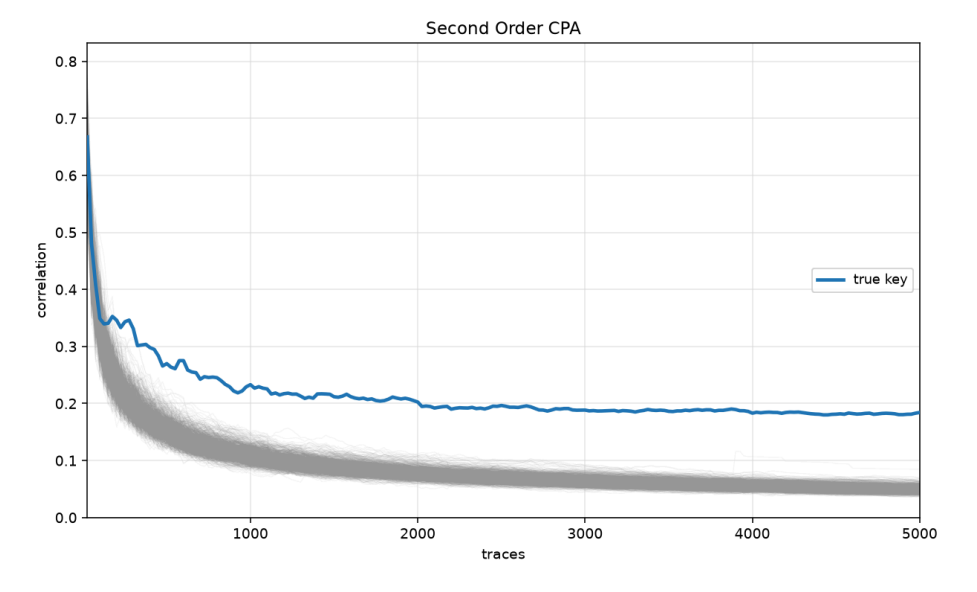
The correct coefficient wins decisively. In our experiment, the true key reaches rank 0 after about 200 traces.

Conclusion

Masking did its job at first order. Looking at any single sample, the secret is invisible: the SNR is flat, and the 40-trace first-order attack that worked on the unprotected implementation no longer applies.

But first-order security is not the end of the story. The leakage was redistributed into two shares. Each share still leaks on its own, and the centered cross-product recombines the physical leakage in a way the key can influence.

Masking therefore buys meaningful complexity. The attacker must find two leakage points, process the traces jointly, and use a leakage model that matches the second-order measurement. That is a real increase in difficulty, but it is not a wall.

The broader lesson is familiar: a single countermeasure is rarely enough. Robust implementations layer masking with shuffling, which randomizes the order of operations, and desynchronization, which randomizes timing and complicates trace alignment. Each layer multiplies the attacker’s effort. Together, they make this kind of attack far less tractable.

---

Alain Magazin & Karim M. Abdellatif, Ph.D. - Ledger Donjon

Footnotes

1. Emmanuel Prouff, Matthieu Rivain and Regis Bevan, “Statistical Analysis of Second Order Differential Power Analysis”. ↩